Towards Financial World Modeling
- Humzah MerchantUniversity of Chicago
- Alec GuthrieUniversity of Chicago
- Simon MahnsJohns Hopkins University
- Randall BalestrieroBrown University
- Bradford LevyUniversity of Chicago
Financial markets are noisy, complex environments that present unique challenges for representation learning. Motivated by the success of supervised and self-supervised learning in computer vision and language, we explore the extent to which they can learn a world model of financial markets, one useful not only for tasks known in advance, but for auxiliary tasks never seen during training.
1.The Market-1T Dataset
≈1T one-second aggregates, all US equities, 2008–2025. Pending release.
Market-1T spans all equities traded on US markets from 2008 through 2025. Raw quotes and trades are aggregated into one-second intervals, roughly one trillion observations. The base data is mid-frequency; the same aggregations extend to minute, hourly, or daily scales.
Each one-second snapshot carries 11 features, bucketed into three groups:
- Order book state: best bid/ask prices and sizes
- Price summary: open, high, low, close, and VWAP
- Activity: volume and trade count
Experiments focus on a liquid universe, re-calculated monthly from prior-month activity (Price > $5, ADV ≥ $20M).
1.1Why mid-frequency
Prediction problems split by timescale, and each band is driven by something different. We target the mid-frequency regime, minutes to days, where new information arrives, gets priced, and interacts with market dynamics. High frequency is dominated by latency and infrastructure; low frequency is data-starved and macro-driven. Mid-frequency has signal, density, and no dependence on colocation.
| Low-frequency | Mid-frequency | High-frequency | |
|---|---|---|---|
| Timescale | Weeks to months | Minutes to days | Micro- to milliseconds |
| Drivers | Macro trends, fundamentals, real-world events | Information flow, market reactions, short-horizon dynamics | Microstructure, exchange mechanics, latency, execution |
2.Methodology
What we predict, how we crop a trading day, and how LeJEPA learns without labels.
2.1Tasks
The core tasks come from portfolio choice. To pick weights, an investor needs three forecasts: expected return, risk (volatility and covariances), and trading cost. We train models to predict each one, forward return, change in volatility, and change in bid-ask spread, at horizons from 5 minutes to 2 hours. These forecasts are not a trading strategy; they are the inputs a strategy would consume.
- Return (primary evaluation): 5-way classification of 15-minute forward mid-price returns, one bin for zeros, the rest empirical quantiles.
- Volatility change: how much conditional volatility moves, the risk term in the portfolio problem.
- Spread change: how the bid-ask spread moves, a standard proxy for transaction cost.
Supervised models train on these labels directly, one task at a time or all three at once. SSL models see no labels; we read their representations afterward with linear probes on the same targets. We also probe for things finance does not usually label, namely ticker, time of day, and trading day within the month (plus a separate test on SEC-documented manipulation windows). These are nearly uncorrelated with return, volatility, and spread, so a supervised model has no reason to learn them. If a representation predicts them anyway, it is carrying structure beyond the task it was trained for.
2.2Scale and crop
Vision SSL leans on strong augmentation, and the workhorse is random scaling and cropping. We port it to markets. Sample a scale s and a random window of the asset-day, then resize to a fixed token length L. The catch is the resize: instead of interpolating pixels, we re-aggregate the way markets already do, last order book state, OHLC, VWAP, summed volume and trade count.
Global views cover broad intraday structure; local views zoom in on shorter horizons. They are sampled independently and may not overlap, so the encoder has to recognize the same day across different windows, resolutions, and sampling rates. Two global views at L = 2048 with s ∈ [0.5, 1.0]; local views at L = 512 with s ∈ [0.05, 0.5]. This augmentation is the default for LeJEPA, DINO, and BYOL.
2.3How LeJEPA works
LeJEPA is our main self-supervised baseline. It learns in representation space: rather than reconstruct raw prices, it predicts the latent of one view of an asset-day from another. The crop makes the views, the encoder embeds each one, and a predictor maps between them, with no return or volatility labels anywhere.
No labels
The target is another view of the same day, not a return or volatility label.
SIGReg (λ = 0.01)
Spreads the embeddings out so the predictor can't cheat by collapsing everything to one point.
Prediction alone has a trivial solution: map everything to the same point. SIGReg (default λ = 0.01) blocks that collapse by keeping the embedding distribution spread out. The default run is a ViT backbone, learning rate 5×10⁻⁴, six local views, batch size 128. We then freeze the backbone and read it with linear probes on the tasks above, alongside supervised models that did see the labels. On the core tasks the gap is widest at the supervised head and narrows once both are read the same way, by a probe.
3.Evaluation
Strict temporal splits and ΔAUC over a random-init baseline keep the future out.
We adopt a strict temporal evaluation scheme. All hyperparameter selection and training happen on data prior to calendar time t; final models are evaluated strictly after t. Interleaving training and evaluation days introduces look-ahead bias and is disallowed.
Performance is reported as ΔAUC = AUC(trained) − AUC(random-init), averaging the random baseline over 10 initializations. Even a probe on random projections can beat chance.
Rolling multi-regime evaluation samples 32 training months and evaluates on the immediately following month. The primary task is 5-way classification of 15-minute forward mid-price returns, with one bin reserved for zero returns and the rest empirical quantile bins.
4.Results
Supervised heads lead on the named targets; SSL lags there but remembers structure those targets leave out: ticker identity, calendar, and the response to news.
We compare two families. Supervised models learn from labels, predicting future return, volatility change, or spread change from a past window. LeJEPA and the other self-supervised methods learn from views, aligning representations of global and local crops of the same asset-day with no labels.
We evaluate LeJEPA, MAE, CPC, DINO, BYOL, and supervised baselines on the core tasks: return, volatility change, and spread change. Supervised still wins. Across every backbone, the supervised head beats its self-supervised counterpart, and the gap shrinks, but does not close, once we read both with a probe instead of the head.
Among the self-supervised objectives, DINO is the strongest and I-JEPA the weakest. All of them learn nontrivial representations, but none close the gap to LeJEPA or the supervised baselines on these targets.
The tasks also help each other. A model trained on volatility or spread change transfers onto return prediction, and a single backbone with one head per task beats the return-only baseline. The transfer is one-directional: other tasks improve return prediction, but return prediction does not improve them.
ΔAUC per backbone: self-supervised vs supervised
15-minute return, ΔAUC over random init (×100); supervised head on the x-axis, LeJEPA (λ=0.01) on the y-axis.
Below the dashed parity line, the supervised model wins. Against its trained head, every backbone sits well below the diagonal; the gap narrows once both families are read the same way (by a linear probe). Numbers are Table 1; bars are ±1 SE.
| Task | Stronger head | Note |
|---|---|---|
| 15-min return | Supervised | 5-way return bins |
| Volatility change | Supervised | spills onto return |
| Spread change | Supervised | spills onto return |
| Multi-task backbone | Supervised | lifts the return baseline |
4.1What the model remembers
SSL trails on the core tasks but recovers ticker, time-of-day, and calendar structure the return label never asked for.
Beyond the next price move, a representation can also encode where it sits: the asset, the time of day, the point in the month. The figure below is a real t-SNE of market-window embeddings, six stocks from three sectors, one global-view crop per ticker-day, colored by ticker.
Under LeJEPA, the points sort into tight per-ticker islands, structure the return label never asked for. Under Supervised, the same six stocks collapse into a far more undifferentiated cloud. The islands are per-ticker, not per-sector: the two semis, two banks, and two oil majors do not merge. That points to each stock's microstructure fingerprint, not its industry.
4.2When news hits the tape
8-K disclosures shift post-event volatility more than direction.
After news, the largest effect is often on uncertainty rather than the direction of prices. We condition a frozen LeJEPA encoder on SEC 8-K filings and ask whether disclosure content improves predictions of the post-event market.
frozen LeJEPA encoder → event-conditioned predictor → post-event latent
| Post-event target | ΔAUC | Significance |
|---|---|---|
| Volatility change | +0.034 | p < 10⁻³ |
| Signed return | +0.010 | p > 0.18 (n.s.) |
Disclosure content shifts conditional variance more than conditional mean. The contrast survives a scrambled-text control.
5.Smaller findings
Markets here are mostly idiosyncratic and low-dimensional, slow to decay month to month, rankable by the SSL loss itself, and legible around news and manipulation.
Beyond the headline comparison, a few smaller results fill in what these models capture.
Mostly idiosyncratic
Adding IWM, a market-factor proxy, leaves the paired ΔAUC at roughly zero. At this frequency, almost all single-stock movement is idiosyncratic, not systematic.
Low-dimensional
A SIGReg projector of dimension 32 is optimal, and 4–8 already work. Market structure is far lower-dimensional than images, echoing classical factor models.
The loss ranks the models
Across 32 months, Corr(loss/λ⁰·⁴, ΔAUC) = −0.698 ± 0.013. LeJEPA's own training loss tracks downstream quality, so models can be selected without labels.
DINO leads the rest
Among the non-LeJEPA objectives, DINO is strongest and I-JEPA weakest. All are nontrivial; none close the gap to LeJEPA or supervised on the core tasks.
5.1Memory holds up over time
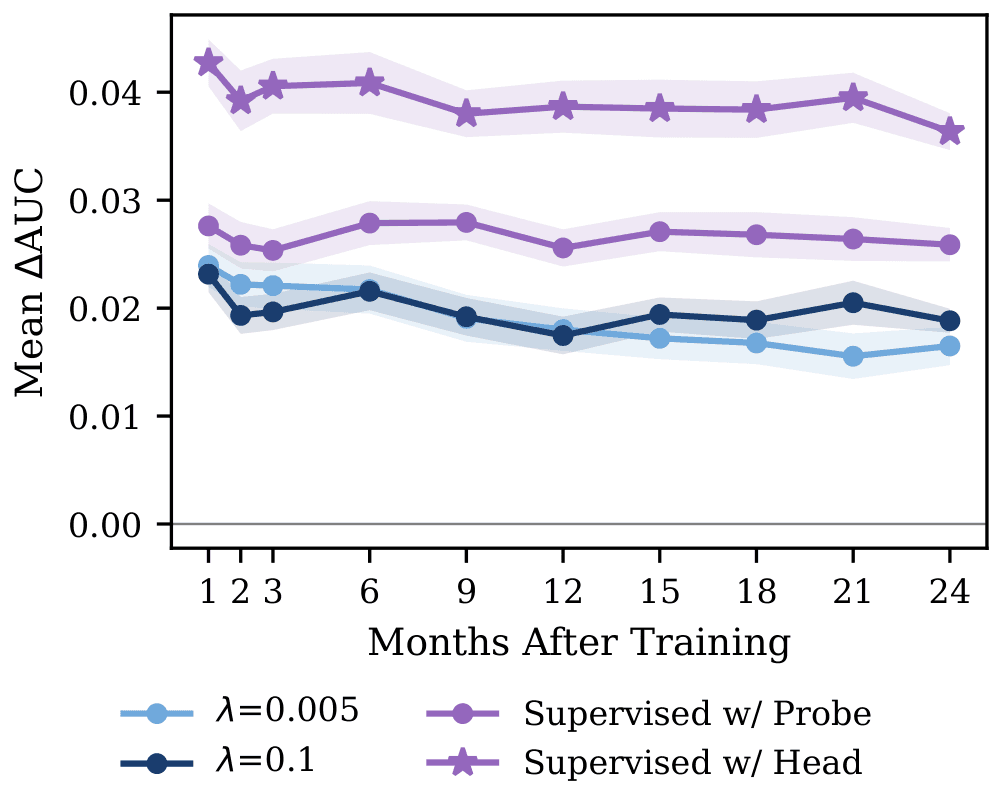
Push the probe from t+1 out to t+24 and performance barely moves after the second month.
By default a model is trained on month t and probed on t+1. Extending the probe to t+24, with the supervised head held fixed, performance is largely flat after the second month. The most extreme near-optimal regularizations we test (λ = 0.005 and λ = 0.1) do not change the picture.
5.2Reading manipulation zero-shot
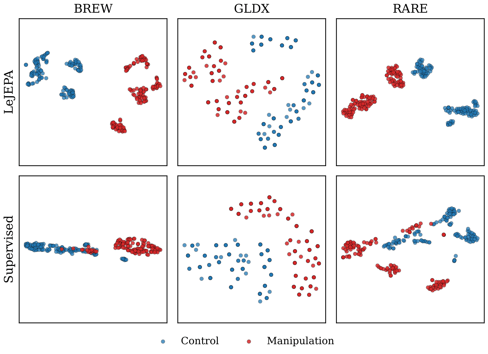
Frozen representations separate SEC-documented manipulation windows from matched controls.
We pull documented manipulation windows from SEC enforcement actions, cases where a participant acted to move price away from fundamentals, and compare them against control periods on other trading days. With no fine-tuning, representations from both LeJEPA and the Supervisedbackbone separate the two, consistent with manipulation's goal of influencing returns.
5.3What a reconstruction looks like
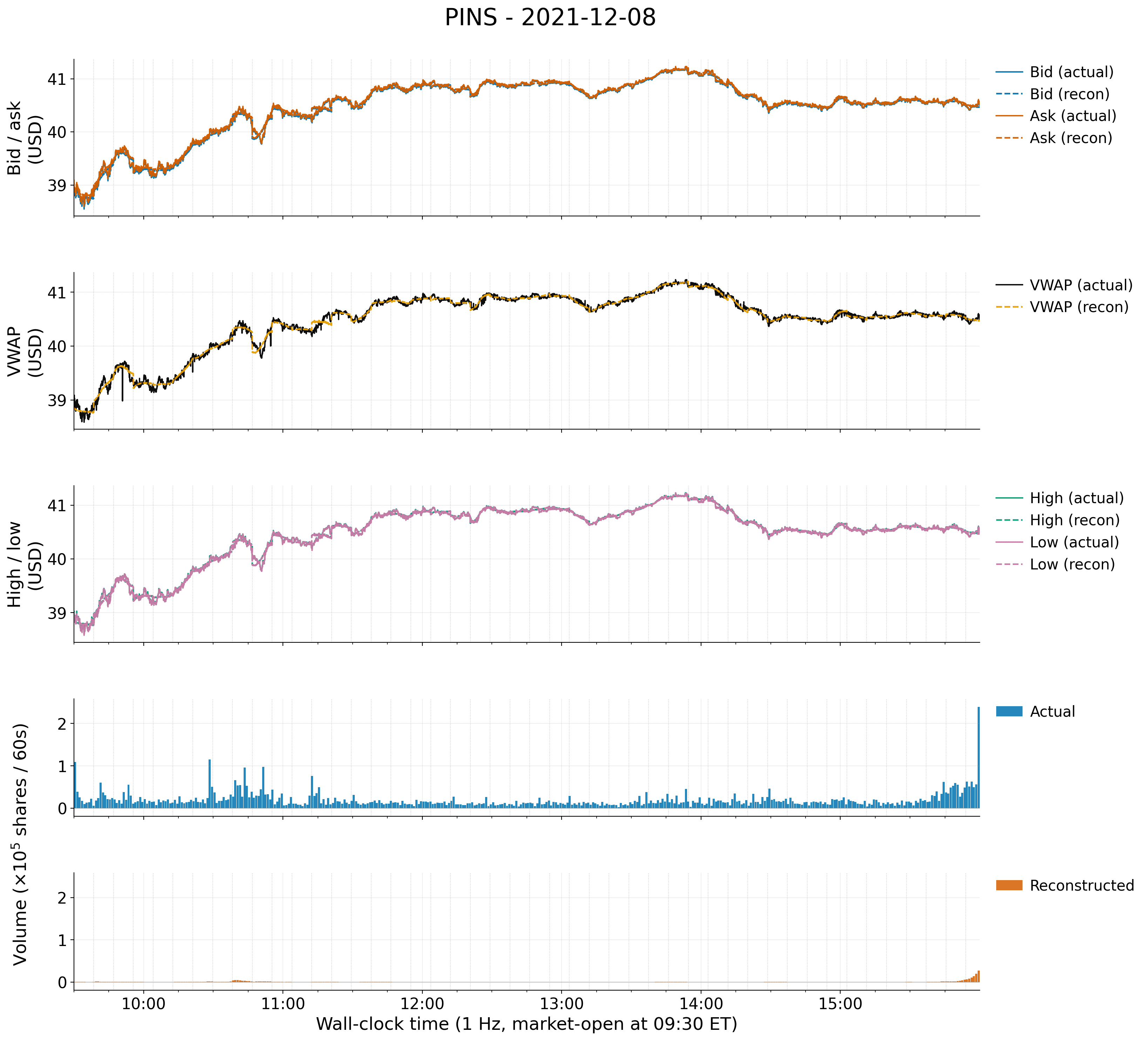
Input-space methods rebuild the raw tape; a sanity check on what the encoder keeps.
Input-space objectives such as the masked autoencoder reconstruct the raw order-book and trade series rather than a latent. The reconstructions are a check on what the encoder retains across a full trading day.
6.When the market changes
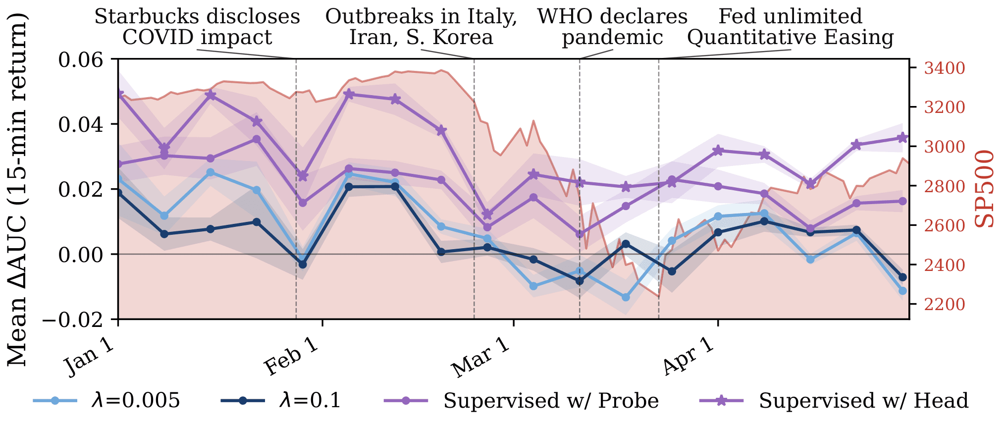
Evaluated across regimes from 2008 to 2025, not a single month, including the early-COVID shock.
The evaluation has to hold across many regimes rather than a single month, which is why Market-1T spans 2008 through 2025.
Marker fill encodes severity (filled = crisis, hollow = calm). Models are trained on month t and evaluated forward; performance is reported across the full series so no single favorable regime drives the result.
During the early-COVID shock, predictive ability shifts around the major turning points.
Technical detailHide detail
Models trained and probed on month t−12 are evaluated through early 2020, sampling one global view per day aggregated to a weekly mean. In contrast, early 2019 was a smooth, upward market. Predictive ability tends to change after pandemic turning points (WHO declaration, Fed QE, market drawdowns).
7.Future work
An illustrative foundation and dataset for further exploration, with disclaimers on scope.
This work is a foundational step, well short of a full market world model, plus a dataset to build on. The longer-term aim is counterfactual policy analysis, the kind a central bank would use.
7.1Disclaimers
High AUC is not profit; it says nothing about returns after execution, transaction costs, latency, sizing, and risk constraints. The study covers single-asset representations only, leaving cross-asset structure and portfolio interactions unexplored. These representations could be misused for manipulation or surveillance evasion, so current data is withheld. Conclusions are limited to US equities and may not transfer to other assets, markets, or regulatory environments.
Citation
@article{merchant2026financial,
  title   = {Towards Financial World Modeling},
  author  = {Merchant, Humzah and Guthrie, Alec and Mahns, Simon
             and Balestriero, Randall and Levy, Bradford},
  journal = {INSERT ARXIV LINK},
  year    = {2026},
}